SOMViz

Today’s mechanical design industry is becoming increasingly complex due to many factors including, but not limited to budget cuts and higher performance expectations. When attempting to design for new objectives, designers must first understand the scope of the problem, and understand the design from an analytical standpoint. However, often problems are becoming so complex that this is not possible without the assistance of computer simulation and modeling. Due to human visual capabilities, data visualization has become a commonly used technique to forego some of the problems introduced by this growing data complexity. SOMViz (Self-Organizing Map Visualization) is an application giving designers and engineers the ability to extract characteristics and trends of high-dimensional data using a directly interpretable 2D visualization of what would otherwise be impossible for a human to cognitively make sense of. Self-Organizing Map (SOM) The core algorithm of SOMViz comes from the Kohonen Self-Organizing Map (SOM). Considered a subset of neural networks, the SOM uses an unsupervised, winner-takes all learning strategy in combination with a time varying, gaussian-based neighborhood update in order to structure a lattice of nodes in such a way to best represent the data set it is being trained on. The “map”, while lending itself to higher dimensions, is often created in a 2D structure due to its ease of interpretation for the human visual system. An example map structure is shown in Figure 1.

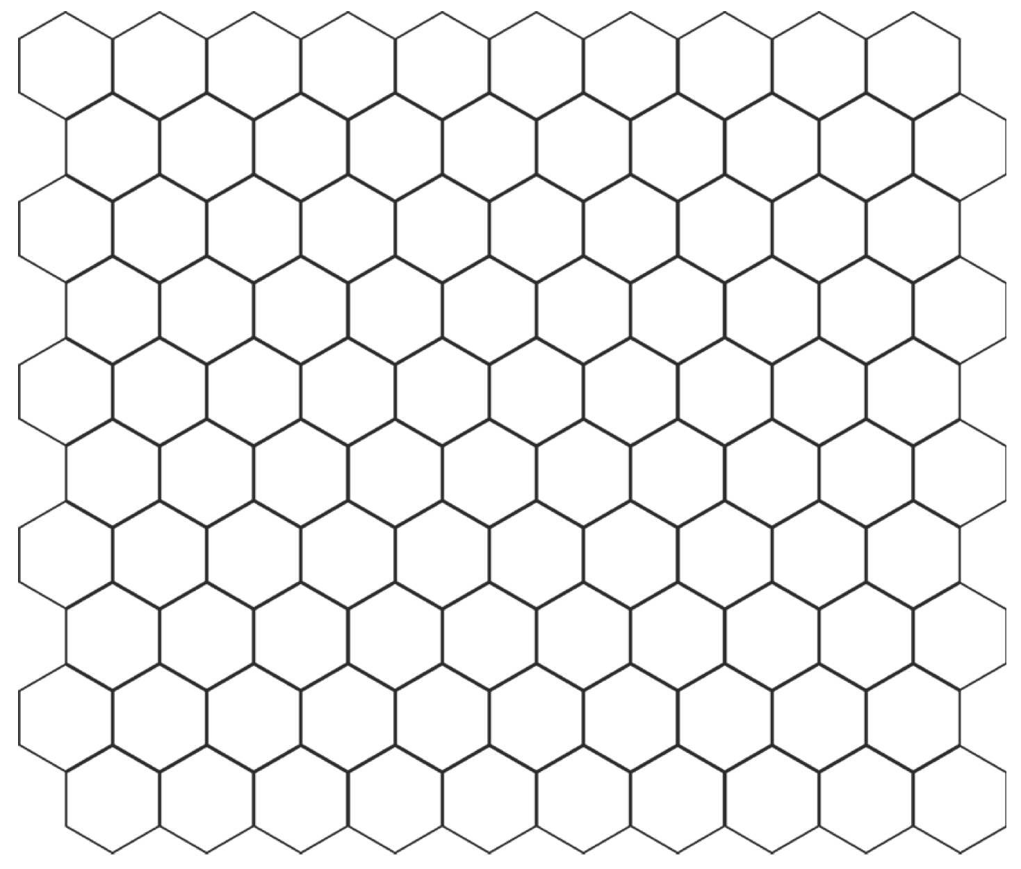
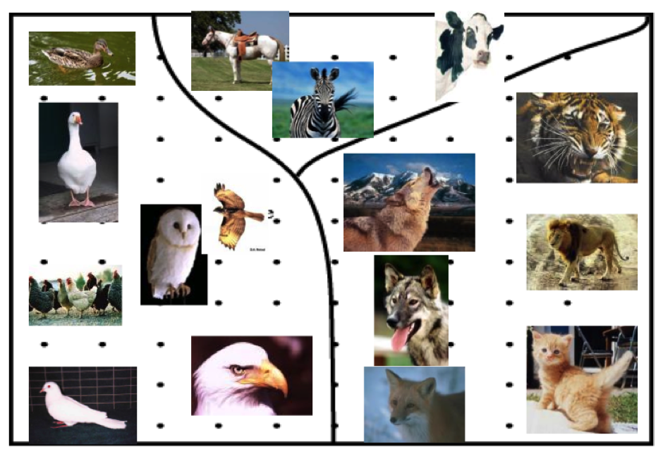
Once an empty map has been initialized, the next step is the training of the map. During this phase, the algorithm runs through a pre-defined number of epochs or generations in Figure 1: Example SOM layout. Order to fit the map to the data. Each epoch of the training consists of “placing” each data point from the set into the map. This placement consist of two steps. First, the node most representative of the data point is found by determining the node of smallest Euclidean  distance between itself and the data point. Once this is complete, the second step, a neighborhood update is performed. During the neighborhood update, the surrounding “neighbors” of the winning node found in the previous step are updated to more closely represent the data point that is being passed in. As this process continues, this neighborhood that is influences by the winning nodes becomes smaller and smaller. Additionally, the amount that the neighborhood “learns” to represent each data point being passed in decreases. By this combination of decreasing the neighborhood influence and decreasing amount of the learning throughout the training, the map becomes more and more refined, resulting in a visualization that has clustered itself into groups of similar dimensional qualities. As an example, Figure 2 shows the result of a SOM trained using the qualities of animals (e.g. [has four legs], [likes to fly]). What the reader may already see is that the SOM has grouped the animals into three major categories: 1) birds 2) hunters 3) peaceful species. The important point to note is that the map is purely training on qualities, it has no sense of a “cat” or a “cow”. In this way, when applied to mechanical design, very complex data can be clustered in such a way that humans would not likely have been capable.

Contextual Self-Organizing Map (CSOM)

Results produced by the training continue to hold a direct mapping back to the underlying data it was initially trained on. Because of this, by using an additional, “contextual” phase in addition to the core SOM algorithm, a visual map can be produced relating underlying characteristic design data to objective (performance) data. To produce this result, the contextual SOM (CSOM) builds upon the SOM by adding an additional step following training. Once training is complete, each data point contained in the data set is passed into the map one final time. Like the procedure for the SOM, the winning node is found for each data point using least Euclidean distance. In a CSOM, however, instead of updating the neighborhood surrounding the winning node, a label representing the current data point is left in the winning node. An example of this “label” is the images that were added following training of the animal data as shown above. While the map was not trained on the image, this image can be used to show the physical interpretation of the characteristics underlying the data. Once this happens, and assuming the data set is larger than the number of nodes in the map, each of the nodes will end up with more than one label contained within itself. Using this, statistics can be found regarding each of the grouped labels found in each resulting map node. Namely, mean, standard deviation, and minimum value of the data points found within each map node can be found. By coloring the nodes to represent these qualities, designers are able to get a quick and interpretable understanding of trends within the data that would otherwise be impossible to directly extract.

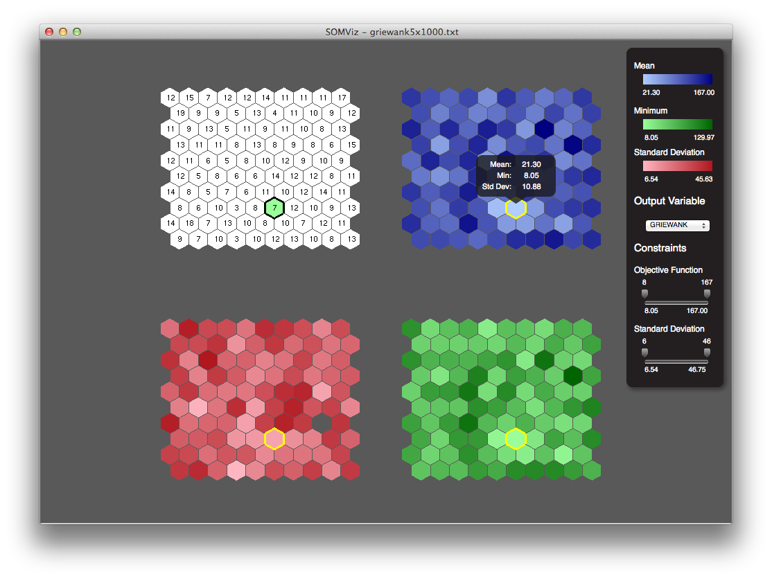
Figure 3 shows an example of the resulting structure of SOMViz following training of a five-dimensional academic data set known as the Griewank Function. The four maps shown are as follows: TL – Count, TR – Mean, BL – Standard Deviation, BR – Minimum Value. It should be noted that the count map (TL) simply shows the number of labels that ended up in that particular node, and were therefore used to calculate the values for each of the remaining three maps. In order to create the visual shown, colors are interpolated from high to low values in each statistical category such that a light color represents a low label value, while a dark color represents a high label value. By providing this visual, a designer can make suggestions as to what the internal behavior of a data set actually looks like. For example, in Figure 2, one might suggest that because the selected node (the node surrounded by a yellow border) contains light blue representing low mean, light red representing low standard deviation, and lightgreen representing low minimum value, the data in this area of the designers trade space is in-fact well-behaved (low standard deviation) around a desirable area (low mean and minimum value) in the design space, as is often the desired qualities of a design.

Summary

While other methods have proven very effective in understanding complex data, very few have shown promise with directly interpretable, n-dimensional data. SOMViz is a step in this direction, but much work undoubtedly remains in this very difficult problem area of mechanical trade space visualization. If more detail is desired, please refer to the following publications:

1. Nekolny, B., Richardson, T., and Winer, E., “Visual Design Space Exploration using Contextual Self-Organizing Maps,” 13th AIAA/ISSMO Multidisciplinary Analysis and Optimization Conference, AIAA 2010, Fort Worth, TX, USA, September 13-15, 2010.

2. Richardson, T., and Winer, E., “Visually Exploring a Design Space Through the Use of Multiple Contextual Self-Organizing Maps,” Proceedings of the ASME 2011 International Design Engineering Technical Conferences & Computers and Information in Engineering Conference, IDETC/CIE 2011, Washington, DC, USA August 29-31, 2011.

3. Holub, J., Richardson, T., Dryden, M., La Grotta, S., and Winer, E., “Contextual Self-Organizing Map Visualization to Improve Optimization Solution Convergence,” 14th AIAA/ISSMO Multidisciplinary Analysis and Optimization Conference, AIAA 2012, Indianapolis, IN, USA, September 17-19 2012.